Modeling Auto insuarance using Machine Learning : Xgboost

insurance

xgboost

explainable machine learning

Data Driven

Published

30 January 2024

Glimpse of the data

First 6 rows of bloodPressure data
INDEX	TARGET_FLAG	TARGET_AMT	KIDSDRIV	AGE	HOMEKIDS	YOJ	INCOME	PARENT1	HOME_VAL	MSTATUS	SEX	EDUCATION	JOB	TRAVTIME	CAR_USE	BLUEBOOK	TIF	CAR_TYPE	RED_CAR	OLDCLAIM	CLM_FREQ	REVOKED	MVR_PTS	CAR_AGE	URBANICITY
1	0	0	0	60	0	11	$67,349	No	$0	z_No	M	PhD	Professional	14	Private	$14,230	11	Minivan	yes	$4,461	2	No	3	18	Highly Urban/ Urban
2	0	0	0	43	0	11	$91,449	No	$257,252	z_No	M	z_High School	z_Blue Collar	22	Commercial	$14,940	1	Minivan	yes	$0	0	No	0	1	Highly Urban/ Urban
4	0	0	0	35	1	10	$16,039	No	$124,191	Yes	z_F	z_High School	Clerical	5	Private	$4,010	4	z_SUV	no	$38,690	2	No	3	10	Highly Urban/ Urban
5	0	0	0	51	0	14	NA	No	$306,251	Yes	M	<High School	z_Blue Collar	32	Private	$15,440	7	Minivan	yes	$0	0	No	0	6	Highly Urban/ Urban
6	0	0	0	50	0	NA	$114,986	No	$243,925	Yes	z_F	PhD	Doctor	36	Private	$18,000	1	z_SUV	no	$19,217	2	Yes	3	17	Highly Urban/ Urban
7	1	2946	0	34	1	12	$125,301	Yes	$0	z_No	z_F	Bachelors	z_Blue Collar	46	Commercial	$17,430	1	Sports Car	no	$0	0	No	0	7	Highly Urban/ Urban

Note

Comments

the data looks really dirty with a lot of bad formatting

Data cleaning

out_new<-out_new %>%
  select(-INDEX) |> 
  mutate(INCOME = as.numeric(gsub('[$,]','',INCOME)),
         HOME_VAL = as.numeric(gsub('[$,]','',HOME_VAL)),
         BLUEBOOK = as.numeric(gsub('[$,]','',BLUEBOOK)),
         OLDCLAIM = as.numeric(gsub('[$,]','',OLDCLAIM)),
         PARENT1 = tolower(gsub('[z_<]','', PARENT1)),
         MSTATUS = tolower(gsub('[z_<]','', MSTATUS)),
         SEX = tolower(gsub('[z_<]','', SEX)),
         EDUCATION = tolower(gsub('[z_<]','', EDUCATION)),
         JOB = tolower(gsub('[z_<]','', JOB)),
         CAR_USE = tolower(gsub('[z_<]','', CAR_USE)),
         CAR_TYPE = tolower(gsub('[z_<]','', CAR_TYPE)),
         RED_CAR = tolower(gsub('[z_<]','', RED_CAR)),
         REVOKED = tolower(gsub('[z_<]','', REVOKED)),
         URBANICITY = tolower(gsub('[z_<]','', URBANICITY)))
colnames(out_new) <- tolower(colnames(out_new))
dict <- read_xlsx('DataDictionary_Insurance.xlsx')
knitr::kable(dict, format = 'pandoc')

VARIABLE NAME	DEFINITION	THEORETICAL EFFECT
INDEX	Identification Variable (do not use)	None
TARGET_FLAG	Was Car in a crash? 1=YES 0=NO	None
TARGET_AMT	If car was in a crash, what was the cost	None
AGE	Age of Driver	Very young people tend to be risky. Maybe very old people also.
BLUEBOOK	Value of Vehicle	Unknown effect on probability of collision, but probably effect the payout if there is a crash
CAR_AGE	Vehicle Age	Unknown effect on probability of collision, but probably effect the payout if there is a crash
CAR_TYPE	Type of Car	Unknown effect on probability of collision, but probably effect the payout if there is a crash
CAR_USE	Vehicle Use	Commercial vehicles are driven more, so might increase probability of collision
CLM_FREQ	#Claims(Past 5 Years)	The more claims you filed in the past, the more you are likely to file in the future
EDUCATION	Max Education Level	Unknown effect, but in theory more educated people tend to drive more safely
HOMEKIDS	#Children @Home	Unknown effect
HOME_VAL	Home Value	In theory, home owners tend to drive more responsibly
INCOME	Income	In theory, rich people tend to get into fewer crashes
JOB	Job Category	In theory, white collar jobs tend to be safer
KIDSDRIV	#Driving Children	When teenagers drive your car, you are more likely to get into crashes
MSTATUS	Marital Status	In theory, married people drive more safely
MVR_PTS	Motor Vehicle Record Points	If you get lots of traffic tickets, you tend to get into more crashes
OLDCLAIM	Total Claims(Past 5 Years)	If your total payout over the past five years was high, this suggests future payouts will be high
PARENT1	Single Parent	Unknown effect
RED_CAR	A Red Car	Urban legend says that red cars (especially red sports cars) are more risky. Is that true?
REVOKED	License Revoked (Past 7 Years)	If your license was revoked in the past 7 years, you probably are a more risky driver.
SEX	Gender	Urban legend says that women have less crashes then men. Is that true?
TIF	Time in Force	People who have been customers for a long time are usually more safe.
TRAVTIME	Distance to Work	Long drives to work usually suggest greater risk
URBANICITY	Home/Work Area	Unknown
YOJ	Years on Job	People who stay at a job for a long time are usually more safe

# test <- read_csv('logit_insurance_test.csv')

Explanatory data analysis

Visualise the target variable

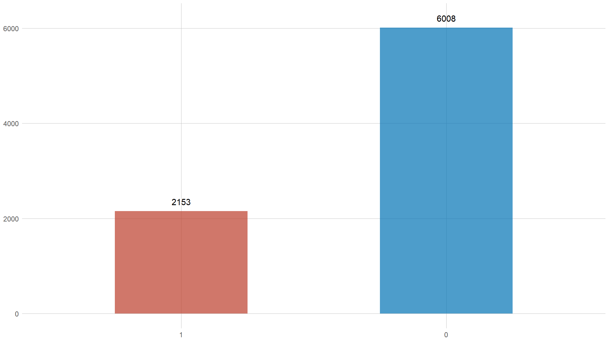
our dataset is not really balanced !!

Relationship between `target flag` and `car type`

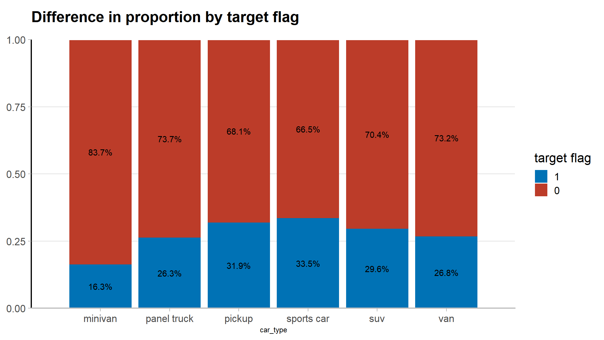
Note

sports cars are at a high risk of being involved in car accidents

distribution of target by education

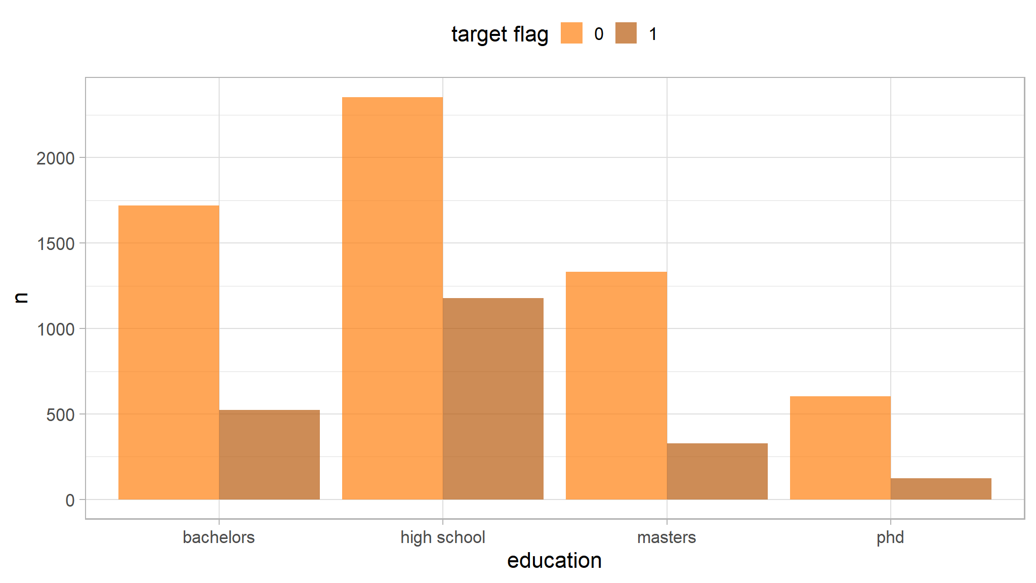
Note

the greatest proportion of those involved in accidents were students in high school

Relationship between target flag and job

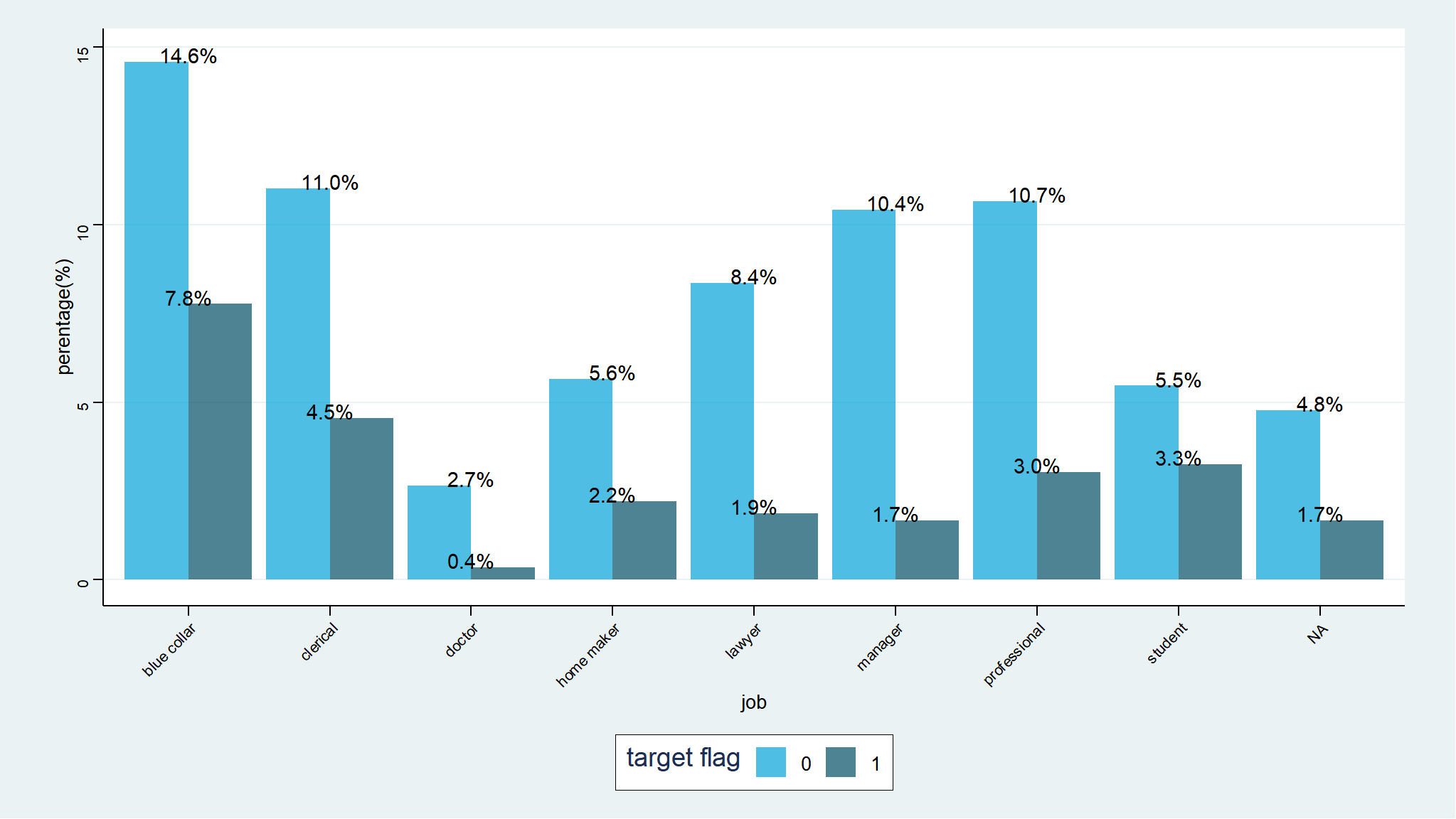
Note

blue collar guys are more prone to accidents

Distribution of numeric variables

Tip

the following are density plots for variables that have been log transformed

numeric_vars <- out_new |> 
  select_if(is.numeric) |> 
  select(-index) |> 
  mutate(target_flag=factor(target_flag,levels=c("0","1"))) |> 
  pivot_longer(!target_flag, names_to = "metric", values_to = "value")

# Density plot
numeric_vars %>% 
  ggplot(mapping = aes(x = value, color = target_flag)) +
  geom_density() +
  scale_x_log10() + 
  labs(color = "") +
  theme(legend.position = "top") +
  facet_wrap(~ metric, scales = "free")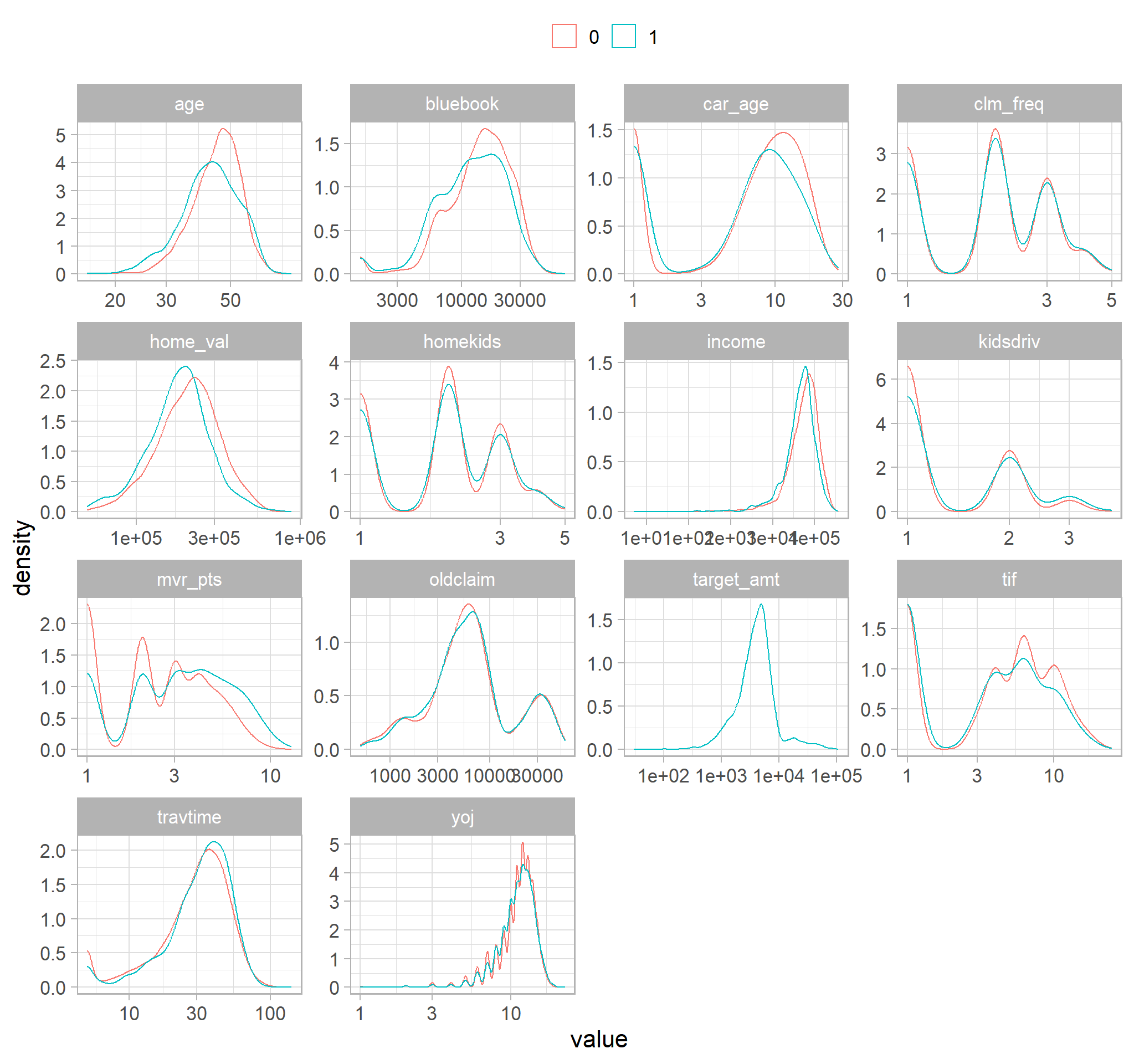


# Use ROc_AUC to determine how well each numeric predictor
# would sway opinions
numeric_vars %>% 
  group_by(metric) %>% 
  roc_auc(target_flag, value, event_level = "second") %>% 
  mutate(metric = fct_reorder(metric, .estimate)) %>% 
  ggplot(mapping = aes(x = .estimate, y = metric)) +
  geom_point() +
  geom_vline(aes(xintercept = .5)) +
  labs(
    x = "AUC estimates of crashing",
    title = "How predictive is each numeric predictor by itself?",
    subtitle = ">.5 means positively influences crashing and <.5 means negatively influences crashing"
  )

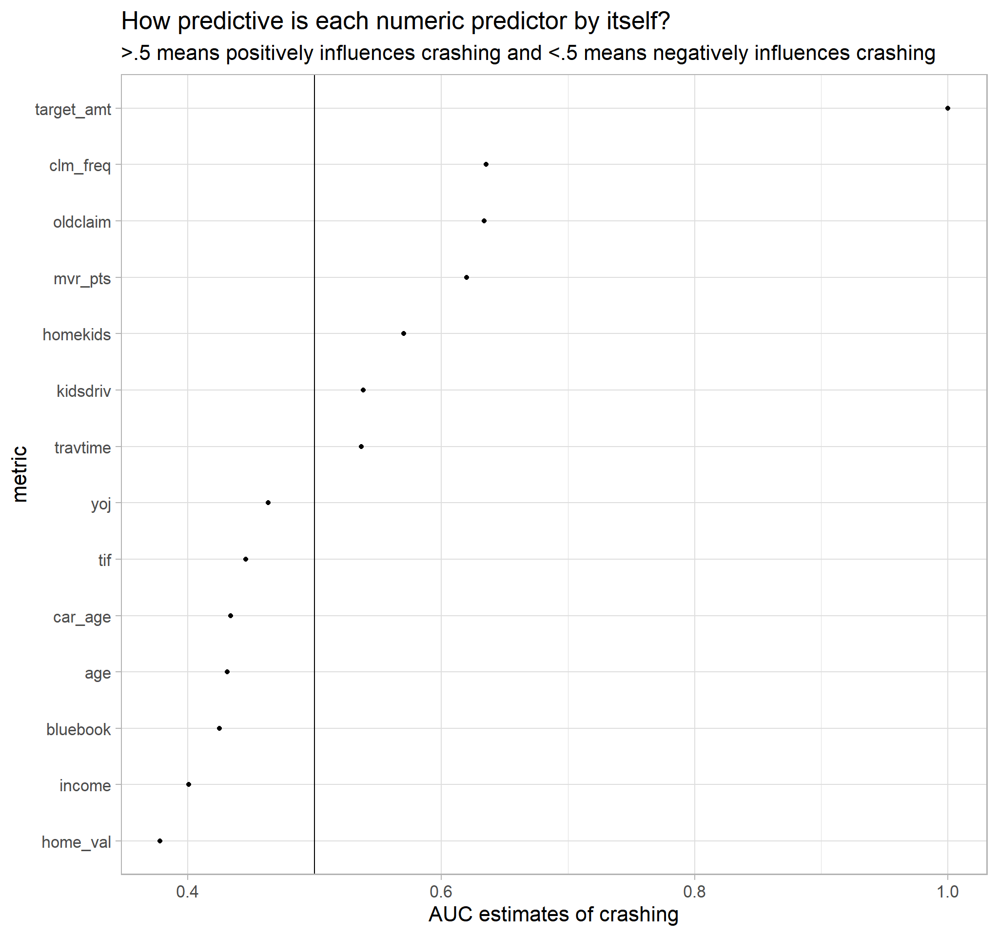
Note

MVR_PTS is greater than .5 hence if you get lots of traffic tickets you tend to get into more crashes
TRAVTIME is greater than .5 hence long drives to work usually suggest greater risk
OLD CLAIM is greater tha .5 suggesting also that if your total payout over the past five years was high ,this suggests future payouts will be high
claim_freq is greater than .5 also suggesting that the more claims you filled in the past the more you are likely to file in the future

Modeling

Specifying a Xgboost model

# Stratified split based on opinion ban
auto_split<-out_new |> 
  mutate(target_flag=as.factor(target_flag))|> 
  initial_split(strata = target_flag, prop = 0.7)

# Obtain train and test sets
train <- training(auto_split)
test <- testing(auto_split)

# Print out observations in each category
glue(
  'The training set has {nrow(train)} observations \n',
  'The testing set has {nrow(test)} observations'
)
#> The training set has 5712 observations 
#> The testing set has 2449 observations

10 Fold cross validation

train_folds <- vfold_cv(data = train, v = 10)

Feature Engineering with recipes

feature engineering entails reformatting predictor values to make them easier for a model to use effectively. The following transformation steps will be done before refining the model further down the line:

One hot encoding: xgboost does not have a means to translate factor predictors to grouped splits. Factor/categorical predictors need to be converted to numeric values (e.g., dummy or indicator variables) for this engine.
Remove zero variance: potentially remove variables that are highly sparse and unbalanced.
Impute missing values:
Normalize/transform: not really required for tree models
Collapse some categorical levels: potentially pool infrequently occurring values into an “other” category.
Upsampling: There is some class imbalance with the survey having more people who agree with ban. > SMOTE requires all variables to be numeric with no missing data. Good thing is that these requirements can and should be handled by previous recipe steps e.g step_impute_mean and step_dummy

prep_juice <- function(recipe){
  recipe |>
    prep() |>
    juice()
}

# Data preprocessing with recipes
boost_recipe <- recipe(target_flag ~., data=train) |>
  step_select(!target_amt) |>
  step_impute_bag(all_numeric_predictors())|>#impute numerical data
  step_impute_mode(all_nominal_predictors())|>#impute nominal data
  step_YeoJohnson(all_numeric_predictors())|># approximate near normal distributions (optional here)
  step_normalize(all_numeric_predictors())|># center and scale numerical vars 
  step_dummy(all_nominal_predictors(), -all_outcomes(), one_hot = TRUE)|># keep ref levels with one hot
  step_nzv(all_numeric_predictors())|># remove numeric vars that have zero variance (single unique value)
  step_corr(all_predictors(), threshold = 0.5, method = 'spearman')|># address collinearity
  themis::step_smote(target_flag) # rebalance the dataset based on the response variable

Create boosted tree model specification

boost_spec <- boost_tree(
  mtry = tune(),
  trees = tune(),
  #min_n = tune(),
  #tree_depth = tune(),
  learn_rate = 0.01,
  #loss_reduction = tune(),
  #sample_size = tune(),
  #stop_iter = tune()
) |>
  set_engine("xgboost") |>
  set_mode("classification")

# Bind recipe and model specification together
boost_wf <- workflow() |>
  add_recipe(boost_recipe) |>
  add_model(boost_spec)

# Print workflow
boost_wf
#> ══ Workflow ════════════════════════════════════════════════════════════════════
#> Preprocessor: Recipe
#> Model: boost_tree()
#> 
#> ── Preprocessor ────────────────────────────────────────────────────────────────
#> 9 Recipe Steps
#> 
#> • step_select()
#> • step_impute_bag()
#> • step_impute_mode()
#> • step_YeoJohnson()
#> • step_normalize()
#> • step_dummy()
#> • step_nzv()
#> • step_corr()
#> • step_downsample()
#> 
#> ── Model ───────────────────────────────────────────────────────────────────────
#> Boosted Tree Model Specification (classification)
#> 
#> Main Arguments:
#>   mtry = tune()
#>   trees = tune()
#>   learn_rate = 0.01
#> 
#> Computational engine: xgboost

Model tuning

Tuning parameter optimization usually falls into one of two categories:
grid_search: when a pre-defined set of parameter values is evaluated and the best set picked. We’ll use a non-regular grid in this case.
When grid search is infeasible or inefficient, iterative methods are a sensible approach for optimizing tuning parameters.
Iterative search or sequential search is when we sequentially discover new parameter combinations based on previous results e.g simulated annealing Using racing methods to perform an efficient grid search.
In racing methods, the tuning process evaluates all hyperparameter combinations on an initial subset of resamples. Based on their current performance metrics, the process eliminates tuning parameter combinations that are unlikely to be the best results using a repeated measure ANOVA model. This is unlike a classical grid search where all models need to be fit across all resamples before any tuning parameters can be evaluated. This efficiently reduces training time.
grid: An integer or data frame. When an integer is used, the function creates a space-filling design with grid number of candidate parameter combinations. Non-regular space-filling designs generally find a configuration of points that cover the parameter space with the smallest chance of overlapping or redundant values.

doParallel::registerDoParallel()
set.seed(2056)
# Evaluation metrics during tuning
eval_metrics <- metric_set(mn_log_loss, accuracy)

# Efficient grid search via racing
xgb_race <- tune_race_anova(
  object = boost_wf,
  resamples = train_folds,
  metrics = eval_metrics,
  
  # Try out 20 different hyperparameter combinations
  grid = 20,
  control = control_race(
    verbose_elim = TRUE
  )
)

beepr::beep(9)
#saveRDS(xgb_race, "smot

# Plot racing results
plot_race(xgb_race)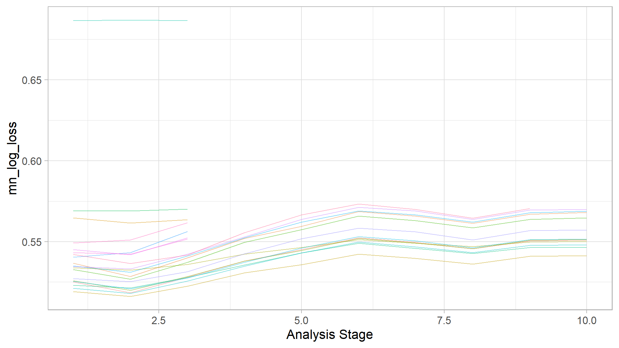

Note

we observe an incremental elimination of tuning parameters that may not have likely improved model perfomance

Accuracy of the models

xgb_race |>
  show_best(metric = "accuracy")
#> # A tibble: 5 × 8
#>    mtry trees .metric  .estimator  mean     n std_err .config              
#>   <int> <int> <chr>    <chr>      <dbl> <int>   <dbl> <chr>                
#> 1     4   741 accuracy binary     0.714    10 0.00803 Preprocessor1_Model04
#> 2     7  1086 accuracy binary     0.710    10 0.00940 Preprocessor1_Model06
#> 3     5   295 accuracy binary     0.709    10 0.00619 Preprocessor1_Model05
#> 4     8   973 accuracy binary     0.709    10 0.00844 Preprocessor1_Model01
#> 5     8  1768 accuracy binary     0.707    10 0.00889 Preprocessor1_Model02

# Plot
xgb_race |>
  collect_metrics() |>
  select(mtry, trees, .metric, mean) |>
  filter(.metric == "accuracy") |>
  pivot_longer(!c(mean, .metric), names_to = "metrics", values_to = "values") |>
  ggplot(mapping = aes(x = values, y = mean)) +
  geom_point(size = 2, color = "darkorange", alpha = 0.7) +
  geom_line(color = "dodgerblue", size = 1.2, alpha = 0.7) +
  labs(y = "accuracy") +
  facet_wrap(vars(metrics), scales = "free_x")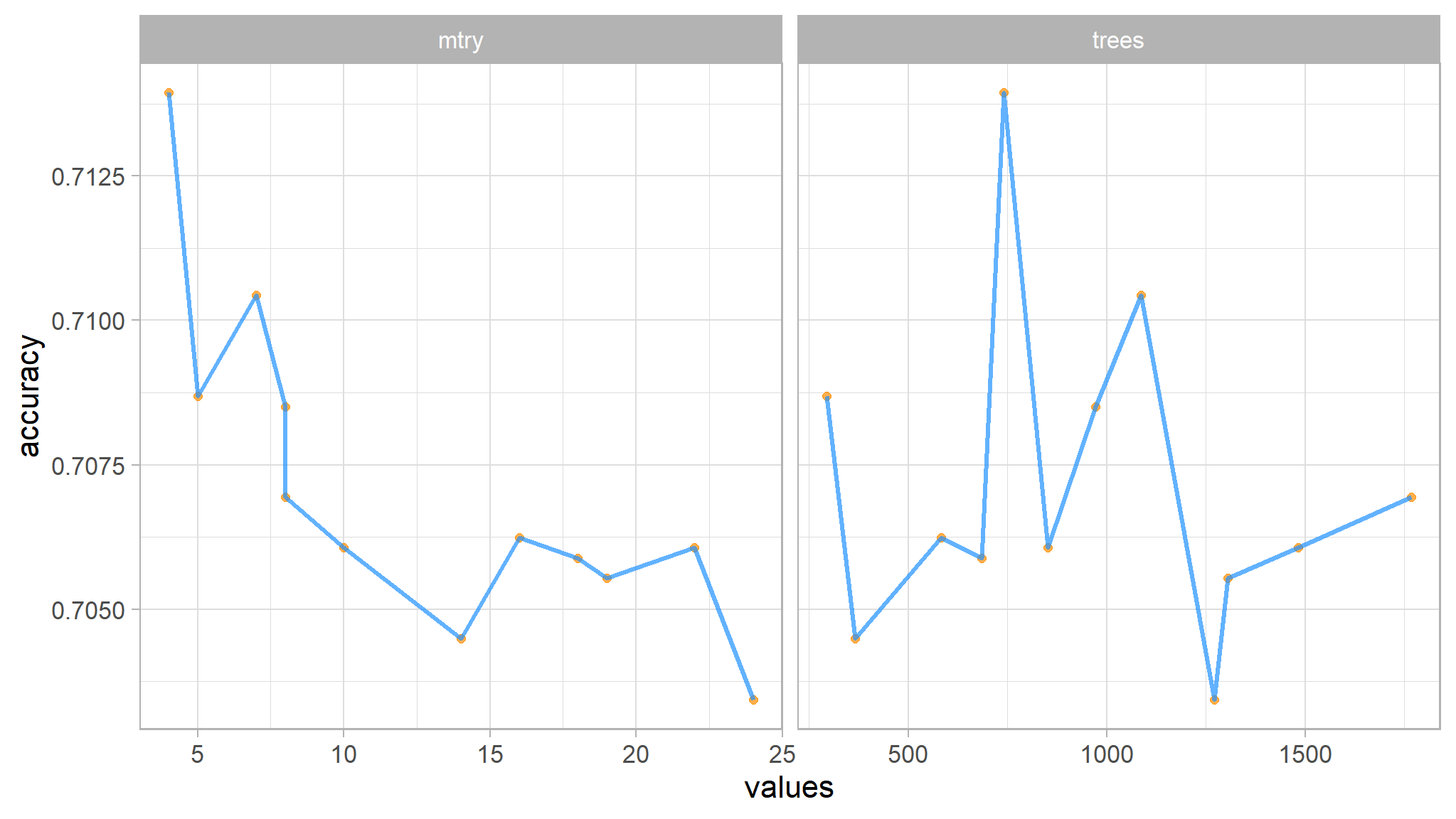

Tip

how accuracy varies with different combinations of mtry and trees

Mean log loss

# Tibble
xgb_race |>
  show_best(metric = "mn_log_loss")
#> # A tibble: 5 × 8
#>    mtry trees .metric     .estimator  mean     n std_err .config              
#>   <int> <int> <chr>       <chr>      <dbl> <int>   <dbl> <chr>                
#> 1     4   741 mn_log_loss binary     0.541    10 0.00784 Preprocessor1_Model04
#> 2    14   367 mn_log_loss binary     0.547    10 0.00747 Preprocessor1_Model09
#> 3    16   584 mn_log_loss binary     0.548    10 0.00860 Preprocessor1_Model11
#> 4     5   295 mn_log_loss binary     0.550    10 0.00546 Preprocessor1_Model05
#> 5     8   973 mn_log_loss binary     0.551    10 0.00904 Preprocessor1_Model01

# Plot
xgb_race |>
  collect_metrics() |>
  select(mtry, trees, .metric, mean) |>
  filter(.metric == "mn_log_loss") |>
  pivot_longer(!c(mean, .metric), names_to = "metrics", values_to = "values") |>
  ggplot(mapping = aes(x = values, y = mean)) +
  geom_point(size = 2, color = "dodgerblue", alpha = 0.7) +
  geom_line(color = "darkorange", size = 1.2, alpha = 0.7) +
  labs(y = "mn_log_loss") +
  facet_wrap(vars(metrics), scales = "free_x")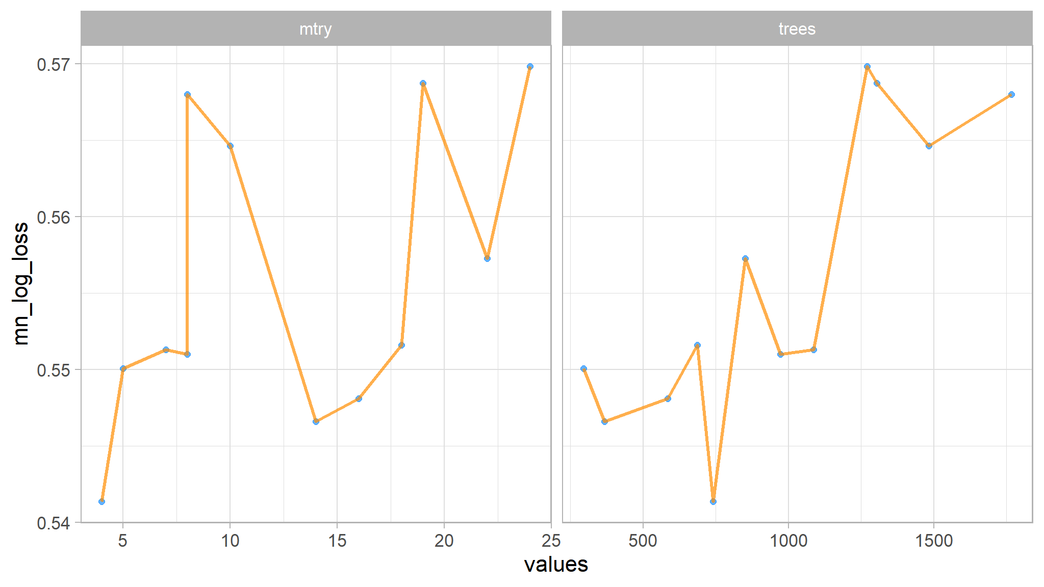

# Finalize workflow
final_boost_wf <- boost_wf |>
  finalize_workflow(select_best(xgb_race, metric = "mn_log_loss" #mn_log_loss
                    ))

# Train then test
xgb_model <- final_boost_wf |>
  last_fit(auto_split, metrics = metric_set(accuracy, recall, spec, ppv, roc_auc, mn_log_loss, f_meas))

# Collect metrics
xgb_model |>
  collect_metrics() 
#> # A tibble: 7 × 4
#>   .metric     .estimator .estimate .config             
#>   <chr>       <chr>          <dbl> <chr>               
#> 1 accuracy    binary         0.710 Preprocessor1_Model1
#> 2 recall      binary         0.684 Preprocessor1_Model1
#> 3 spec        binary         0.785 Preprocessor1_Model1
#> 4 ppv         binary         0.899 Preprocessor1_Model1
#> 5 f_meas      binary         0.777 Preprocessor1_Model1
#> 6 roc_auc     binary         0.819 Preprocessor1_Model1
#> 7 mn_log_loss binary         0.533 Preprocessor1_Model1

Collect metric results

# Plot confusion matrix
xgb_model |>
  collect_predictions() |>
  conf_mat(truth = target_flag, estimate = .pred_class) |>
  autoplot(type = "heatmap")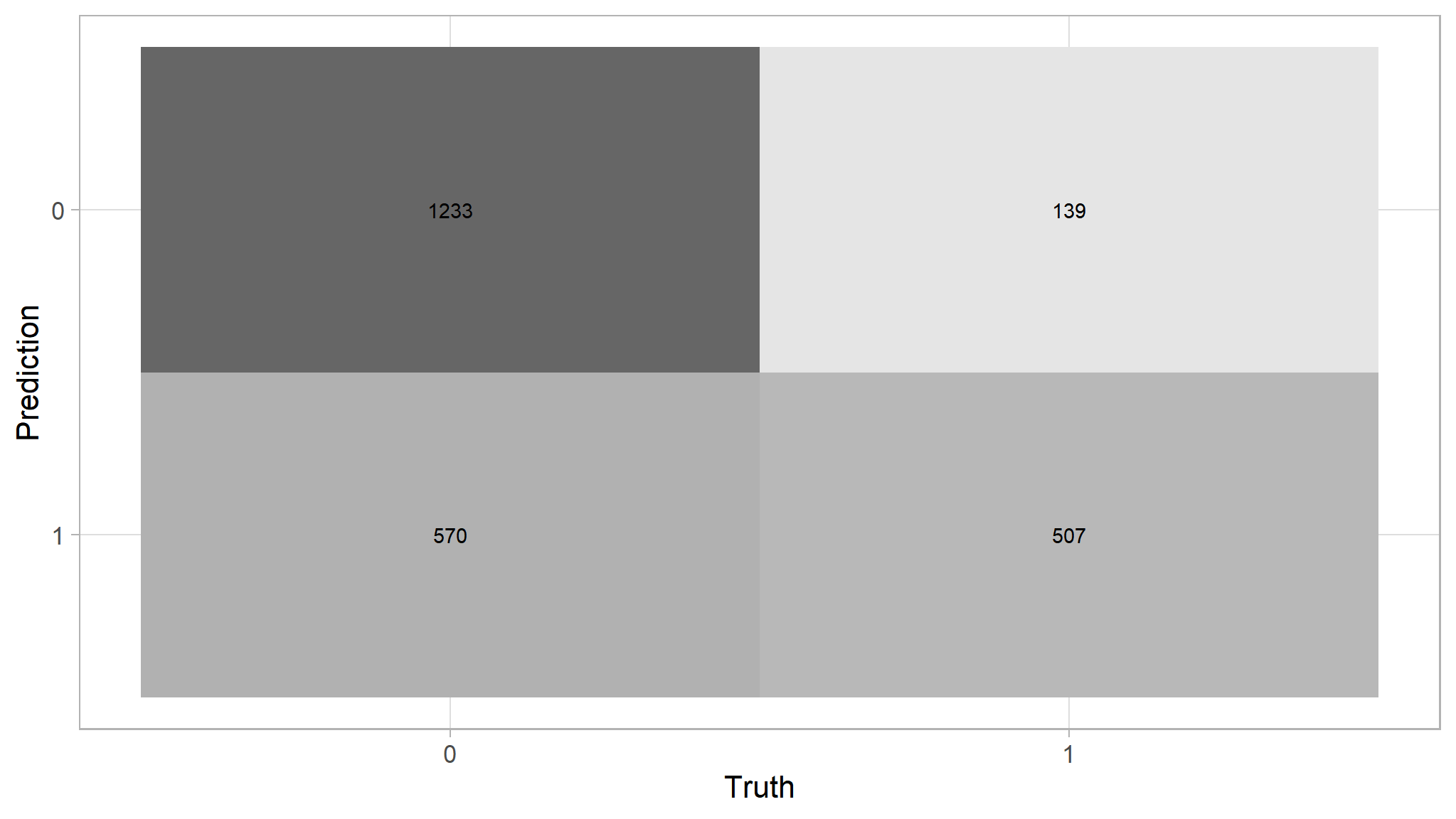


# Prettier?
update_geom_defaults(geom = "rect", new = list(fill = "midnightblue", alpha = 0.7))

xgb_model |>
  collect_predictions() |>
  conf_mat(target_flag, .pred_class) |>
  autoplot()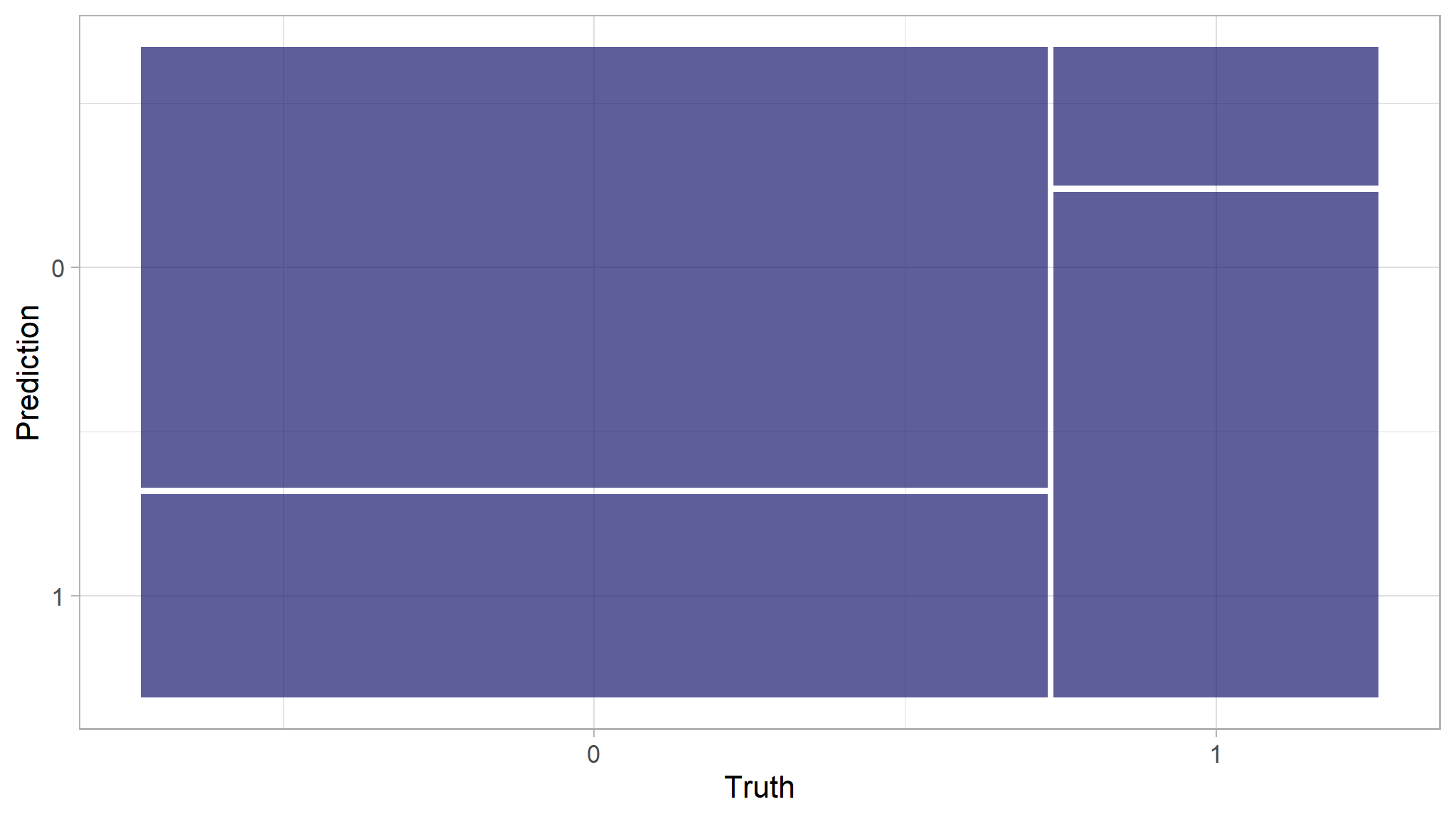


# Extract trained workflow
xgb_wf <- xgb_model |>
  extract_workflow()

The performance metrics considered are:

Recall: TP/(TP + FN) defined as the proportion of positive results out of the number of samples which were actually positive. Also known as sensitivity.
Specificity: TN/(TN + FP) defined as the proportion of negative results out of the number of samples which were actually negative.
Precision: TP/(TP + FP) defined as the proportion of predicted positives that are actually positive. Also called positive predictive value
Accuracy: TP + TN/(TP + TN + FP + FN) The percentage of labels predicted accurately for a sample.
F Measure: A weighted average of the precision and recall, with best being 1 and worst being 0.

Variable importance

Variable Importance/Permutation feature importance plots are one way of understanding which predictor has the largest effect on the model outcomes. The main idea is to measure how much does a model’s performance changes if the effect of a selected explanatory variable, or of a group of variables, is removed. To remove the effect, we use perturbations, like resampling from an empirical distribution or permutation of the values of the variable.If a variable is important, then we expect that, after permuting/shuffling the values of the variable, the model’s performance will worsen. The larger the change in the performance, the more important is the variable. Please see Explanatory Model Analysis and Interpretable Machine Learning

The methods may be applied for several purposes.
Model simplification: variables that do not influence a model’s predictions may be excluded from the model.
Model exploration: comparison of variables’ importance in different models may help in discovering interrelations between the variables. Also, the ordering of variables in the function of their importance is helpful in deciding in which order should we perform further model exploration.
Domain-knowledge-based model validation: identification of the most important variables may be helpful in assessing the validity of the model based on domain knowledge.
Knowledge generation: identification of the most important variables may lead to the discovery of new factors involved in a particular mechanism.

# Load saved model
#xgb_wf <- readRDS("smote_boost_hnwf")
options(scipen = 999)

# Extract variable importance
library(vip)
vi <- xgb_wf |>
  extract_fit_parsnip() |>
  vi()

vi
#> # A tibble: 30 × 2
#>    Variable                       Importance
#>    <chr>                               <dbl>
#>  1 urbanicity_highly.urban..urban     0.148 
#>  2 home_val                           0.106 
#>  3 clm_freq                           0.0796
#>  4 bluebook                           0.0730
#>  5 age                                0.0682
#>  6 mvr_pts                            0.0666
#>  7 travtime                           0.0602
#>  8 index                              0.0549
#>  9 car_type_minivan                   0.0412
#> 10 yoj                                0.0375
#> # ℹ 20 more rows

Let’s represent the above as Variable Importance Plots:

# Make Variable Importance Plots
vi |>
  slice_max(Importance, n = 42) %>%
  mutate(Variable = fct_reorder(Variable, Importance)) %>%
  ggplot(mapping = aes(y = Variable, x = Importance)) +
  geom_point(size = 3, color = "dodgerblue") + 
  geom_segment(aes(y = Variable, yend = Variable, x = 0, xend = Importance), size = 2, color = "dodgerblue", alpha = 0.7 ) +
  ggtitle(paste("Variable Importance plot of top", round(nrow(vi)/2), "variables")) +
  theme(plot.title = element_text(hjust = 0.5))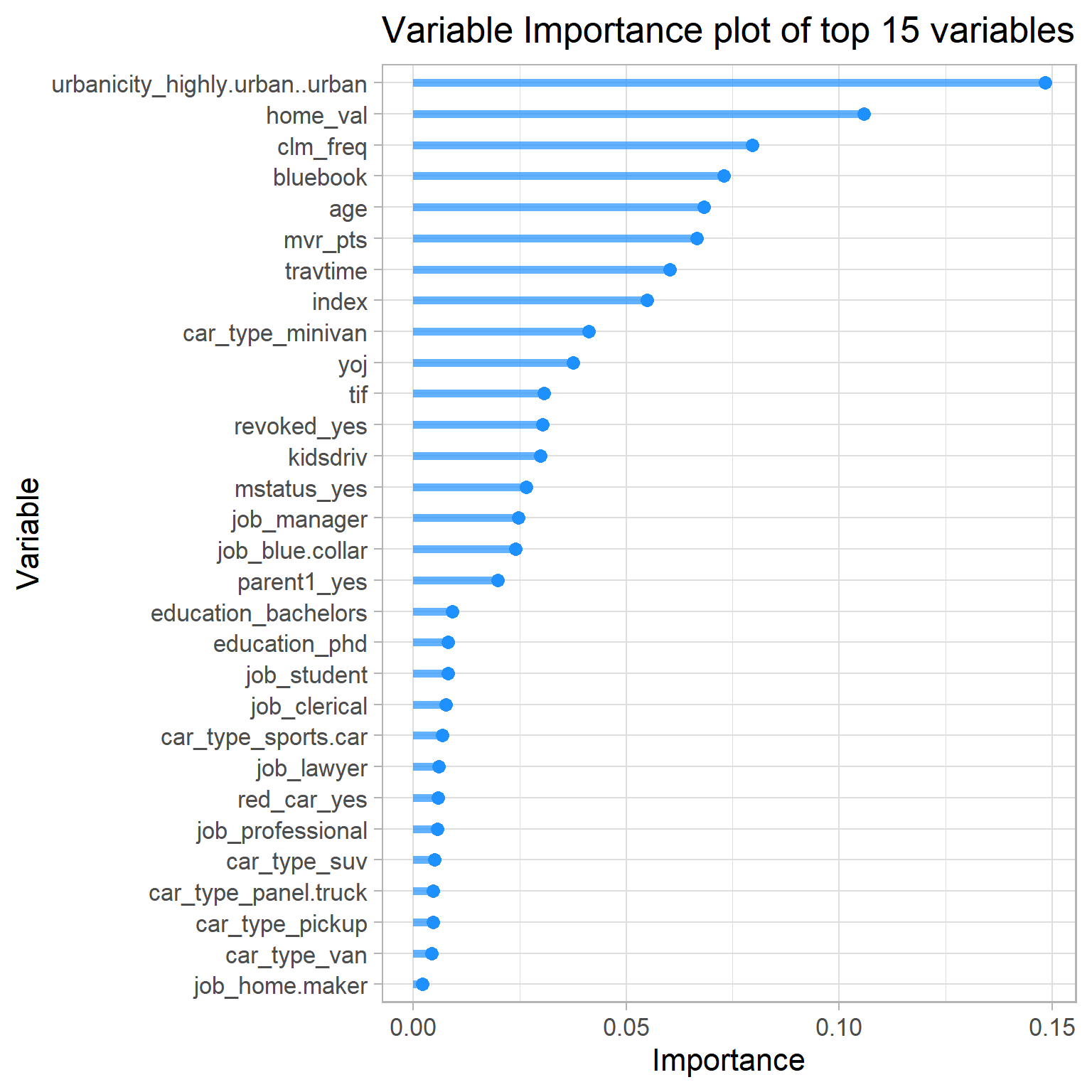

Note

as seen earlier , claim freqency has a significant predictive power
Motor vehicle record points also has some great predictive power just as seen from the individual AUC plot seen earlier
travel time has significant effect as well

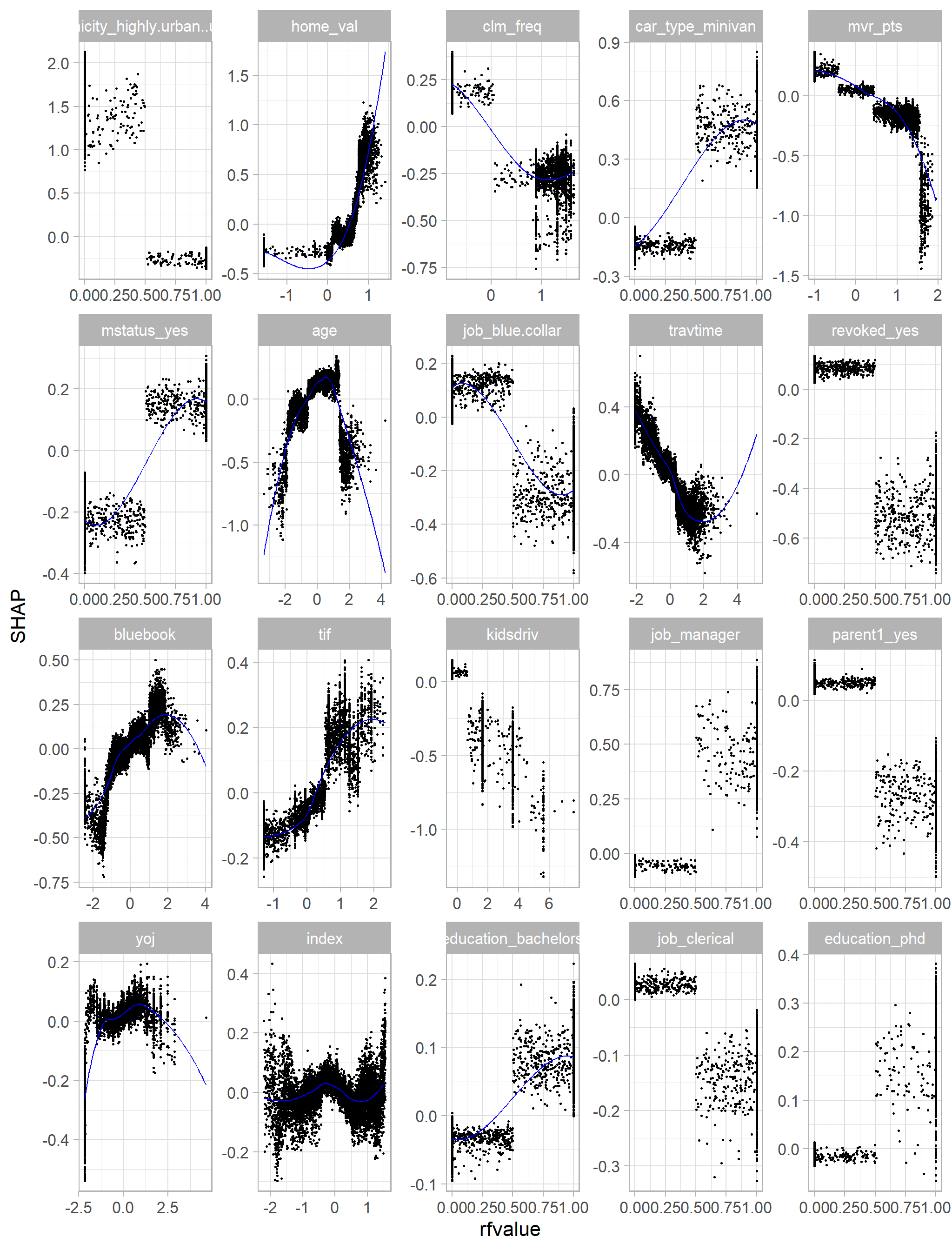
Shapley Additive exPLanations (SHAP)

Tip

SHAP is based on the idea of averaging the value of a variable’s attribution over all (or a large number of) possible orderings.
As such, permutation feature importance is based on decrease in model’s performance with shuffling while SHAP is based on magnitude of feature attributions.
the code below calculates the SHAP values for the top 25 variables ranked by mean SHAP.


# SHAP for xgboost
library(SHAPforxgboost)

# Prepare shap values for plotting. Requires a matrix
opinion_shap <- shap.prep(
  # Actual Boost engine
  xgb_model = xgb_wf |>
    extract_fit_engine(),
  # predictors used to calculate SHAP values
  X_train = boost_recipe |>
    prep() |>bake(has_role("predictor"),
                    new_data = NULL,
                    composition = "matrix"),
  top_n = round(nrow(vi)/2) + 10
  
)

shap.plot.summary(opinion_shap)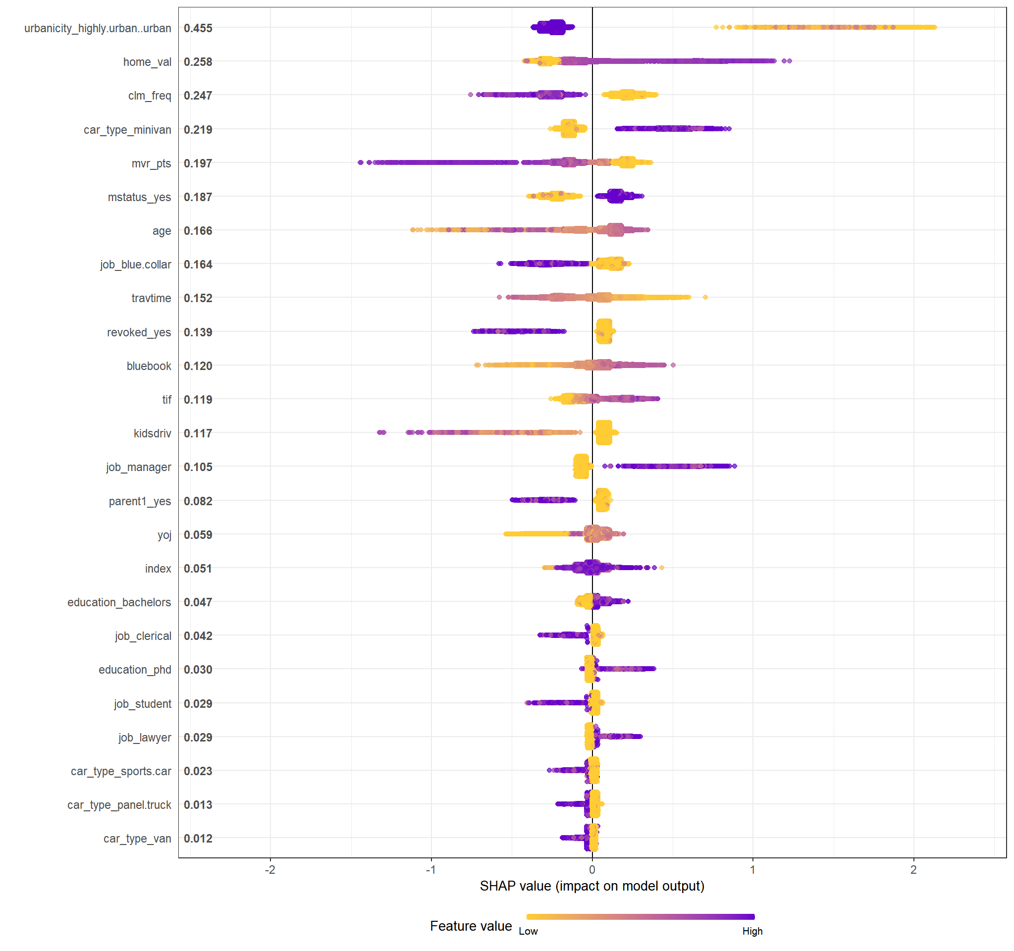

Your regular reminder: All effects describe the behavior of the model and are not necessarily causal in the real world.

opinion_shap |>
  filter(variable %in% (opinion_shap |>distinct(variable) |>slice_head(n = 20) |>pull())) |>
  ggplot(mapping = aes(x = rfvalue, y = value)) +
  geom_point(size = 0.5) +
  geom_smooth(method = "loess", se = F, color = "blue", alpha = 0.7, lwd = 0.4) +
  facet_wrap(vars(variable), scales = "free") +
  ylab("SHAP")

Glimpse of the data

Data cleaning

Explanatory data analysis

Visualise the target variable

Relationship between target flag and car type

distribution of target by education

Relationship between target flag and job

Distribution of numeric variables

Modeling

Specifying a Xgboost model

10 Fold cross validation

Create boosted tree model specification

Accuracy of the models

Mean log loss

Collect metric results

The performance metrics considered are:

Shapley Additive exPLanations (SHAP)

Sources

Relationship between `target flag` and `car type`